Jaesin Ahn, Chaehyeon Lee, Jun-Hyun Bae, Junho Yim, Heechul Jung
Kyungpook National University · LG Energy Solution
8th place out of 1,121 teams
Abstract
Recently, machine unlearning has received considerable attention, in the context of responsible artificial intelligence and privacy regulations. This technical report introduces novel machine unlearning methods, such as stochastic re-initialization, knowledge preserving loss, Gaussian noise, and forget-remember cycle. We present successful unlearning results, validated in the NeurIPS 2023 Machine Unlearning Challenge, accompanied by visualizations of logit distributions and several interim experiments.
Overview
We propose a machine unlearning method that effectively removes the influence of specific data using only the retain set, without accessing the forget set or retraining from scratch.
- Stochastic re-initialization — Randomly select and re-initialize model layers to probabilistically destroy memories of specific data.
- Knowledge preserving — Reproduce the original model’s outputs on the retain set via MSE loss to maintain performance.
- Forget-remember cycles — Repeat forgetting and remembering phases 3–4 times, progressively increasing re-initialization ratio while preserving retain set performance.

Overall architecture. (a) Gaussian noise added to retain set images, (b) random layers selected for stochastic re-initialization, (c) knowledge preserving loss computed between original and unlearning models, (d) steps (a)–(c) repeated for $n$ cycles.
Evaluation
The competition metric is a distribution-based unlearning quality measure, not simple accuracy:
\[\text{Score} = F \times \frac{RA_U}{RA_R} \times \frac{TA_U}{TA_R}\]\(F\) is forgetting quality, \(RA_U / RA_R\) is the retain accuracy ratio (unlearned vs retrained), and \(TA_U / TA_R\) is the test accuracy ratio. Crucially, this metric evaluates the output distribution across 512 independent runs. Since the distribution across runs — not single-run performance — must resemble the retrained model’s distribution, the algorithm requires an appropriate level of randomness.
Method
Stochastic Re-initialization
We randomly select and re-initialize a subset of model layers, then fine-tune on the retain set. While Fisher information matrix (FIM)-based selection is intuitively reasonable, it actually yields lower scores. This is because FIM selects the same layers every run, producing insufficient distributional diversity across 512 runs. Random selection naturally provides this diversity.
FC layers and projection-shortcut layers are excluded from the selection pool as they encode class/resolution information.
Knowledge Preserving Loss
We train the model to reproduce the original model’s outputs on the retain set via MSE loss:
\[\mathcal{L}_{KP} = \mathbb{E}\left[|f_O(\mathbf{I}'_R) - f_U(\mathbf{I}'_R)|^2\right]\]MSE loss (0.0680) outperforms both cross-entropy (0.0653) and L1 loss (0.0326), proving most effective at preserving the original model’s output distribution.
Gaussian Noise Augmentation
Adding Gaussian noise to retain set images provides randomness while achieving robust knowledge preservation. In the ablation, \(\sigma=0.1\) is optimal (0.06532), outperforming both \(\sigma=0.05\) (0.06333) and \(\sigma=0.15\) (0.05907). Vertical flip (0.02505), random crop, and cutout (both 0.00001) distort the data distribution severely, causing scores to plummet, while Gaussian noise yields modest improvement without significantly altering the distribution. The final submission algorithm uses \(\sigma=0.01\) in production, accounting for the 512-run distributional diversity and additional empirical tuning.
Forget-Remember Cycles
Simply increasing the re-initialization ratio causes excessive forgetting. Raising the ratio from 10% to 20% in a single cycle actually decreases the score (0.0680 → 0.0656). Instead, repeating 3–4 cycles of forgetting and remembering progressively increases the effective re-initialization ratio while maintaining retain set performance. This cycle structure is the single largest contributor to performance improvement, with scores rising from a single cycle (0.0680) to 2 cycles (0.0844) to 3 cycles (0.0856).
Algorithm hyperparameters. The 1st algorithm uses 3 cycles of [1, 2, 2] epochs with a cosine learning rate scheduler (\(init\_lr=0.001\)
, \(T\_max=2\)
). The 2nd algorithm uses 4 cycles of [2, 1, 1, 1] epochs with per-epoch learning rates [0.0005, 0.001, 0.001, 0.001, 0.001]. Both algorithms select 6 layers with replacement from the selection pool. The Gaussian noise is sampled from a distribution with zero mean and standard deviation 0.01.
Results
Quantitative
| Model | Score |
|---|---|
| Negrad | 0.0001 (±0.0001) |
| Fine-tune (baseline) | 0.0464 (±0.0031) |
| 1st Algo. (ours) | 0.0939 (±0.0065) |
| 2nd Algo. (ours) | 0.0929 (±0.0051) |
| 1st Algo. (ours, best) | 0.1020 |
| 2nd Algo. (ours, best) | 0.1024 |
Ablation Study
We analyze the contribution of each component sequentially.
Re-initialization.
| Experiment | Score |
|---|---|
| Fine-tune | 0.0496 |
| + Stochastic Re-init (random) | 0.0617 |
| + FIM-based Re-init | 0.0486 |
Data Augmentation (10% Re-init, 3 ep).
| Input Data | Score |
|---|---|
| Clean Image | 0.06172 |
| Vertical Flip | 0.02505 |
| Random Crop | 0.00001 |
| Cutout | 0.00001 |
| + Gaussian Noise (\(\sigma=0.05\) ) | 0.06333 |
| + Gaussian Noise (\(\sigma=0.15\) ) | 0.05907 |
| + Gaussian Noise (\(\sigma=0.1\) ) | 0.06532 |
Loss Functions.
| Loss | Score |
|---|---|
| CE Loss | 0.0653 |
| L1 Loss | 0.0326 |
| MSE Loss | 0.0680 |
Number of Cycles.
| Cycles | Selection Ratio | Score |
|---|---|---|
| 1 (2 ep) | 10% | 0.0680 |
| 1 (2 ep) | 20% | 0.0656 |
| 2 (2-2 ep) | ~20% | 0.0844 |
| 3 (1-2-2 ep) | ~30% | 0.0856 |
Selection Pool (Layer Exclusion).
| Excluded Layers | Selection Ratio | Score |
|---|---|---|
| None | ~30% | 0.0856 |
| FC only | ~30% | 0.0926 |
| FC & Projection-shortcut | ~30% | 0.0969 |
FIM-based re-initialization (0.0486) performs worse than fine-tune only (0.0496). This is because FIM always selects the same critical parameters, producing insufficient distributional diversity across 512 runs. In contrast, random selection (0.0617) naturally generates diverse distributions. Among individual components, the cycle structure (0.0680 → 0.0844 → 0.0856) and layer selection pool restriction (0.0856 → 0.0926 → 0.0969) contribute the largest improvements.
Additionally, layer-wise selection (0.0856) significantly outperforms element-wise selection (0.0575). This is because layer-wise re-initialization appropriately resets functional units of the model, while element-wise selection destroys the learned relationships between parameters within a layer.
Logit Distribution
Comparing logit distributions on the forget set and retain set, our method produces distributions much closer to the retrained model than fine-tuning.
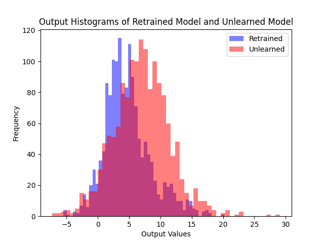
(a) Fine-tune
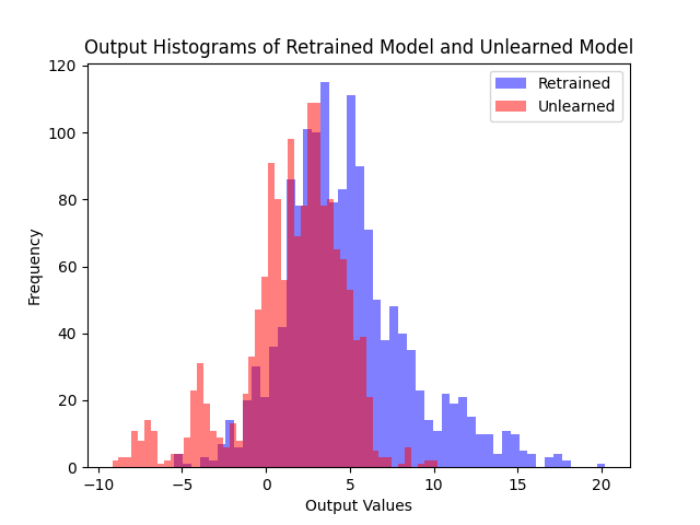
(b) 1st Algo.

(c) 2nd Algo.
Logit distributions on the forget set. Compared to fine-tuning, both of our algorithms produce distributions much closer to the retrained model, with the 2nd algorithm yielding similar shapes to the 1st.
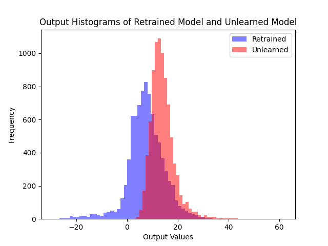
(a) Fine-tune
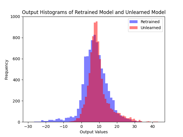
(b) 1st Algo.

(c) 2nd Algo.
Logit distributions on the retain set. Both algorithms maintain similar outputs to the retrained model on the retain set.